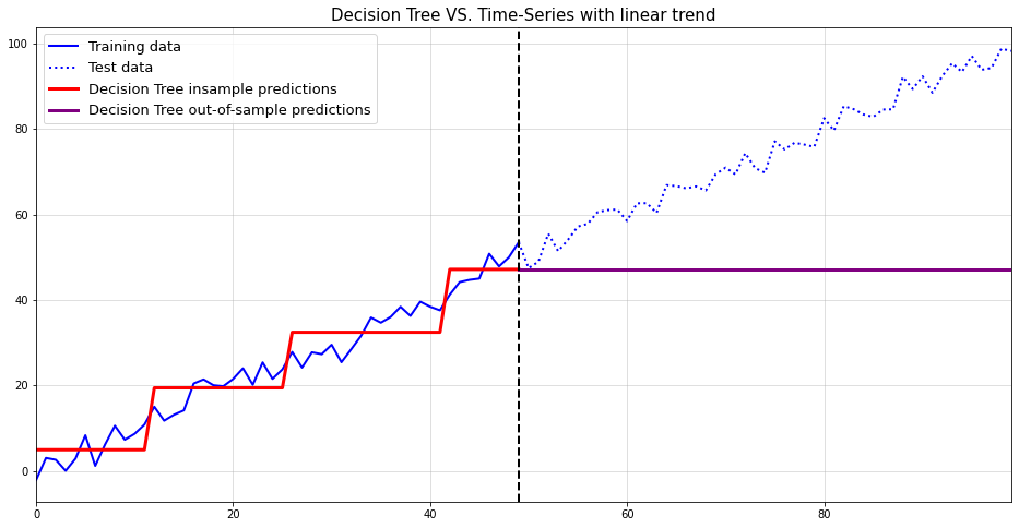
import numpy as npfrom sklearn.tree import DecisionTreeRegressorimport matplotlib.pyplot as plt#create data with linear trendnp.random.seed(123)t = np.arange(100)y = t +2* np.random.normal(size =100)#linear trendt_train = t[:50].reshape(-1,1)t_test = t[50:].reshape(-1,1)y_train = y[:50]y_test = y[50:]tree = DecisionTreeRegressor(max_depth =2)tree.fit(t_train, y_train)y_pred_train = tree.predict(t_train)y_pred_test = tree.predict(t_test)plt.figure(figsize = (16,8))plt.plot(t_train.reshape(-1), y_train, label ="Training data", color="blue", lw=2)plt.plot(np.concatenate([np.array(t_train[-1]),t_test.reshape(-1)]), np.concatenate([[y_train[-1]],y_test]), label ="Test data", color="blue", ls ="dotted", lw=2)plt.plot(t_train.reshape(-1), y_pred_train, label ="Decision Tree insample predictions", color="red", lw =3)plt.plot(np.concatenate([np.array(t_train[-1]),t_test.reshape(-1)]), np.concatenate([[y_pred_train[-1]],y_pred_test]), label ="Decision Tree out-of-sample predictions", color="purple", lw=3)plt.grid(alpha =0.5)plt.axvline(t_train[-1], color="black", lw=2, ls="dashed")plt.legend(fontsize=13)plt.title("Decision Tree VS. Time-Series with linear trend", fontsize=15)plt.margins(x=0)
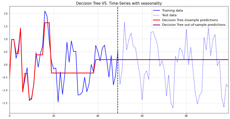
2) Trees cannot handle seasonality
#create data with seasonality np.random.seed(123)t = np.arange(100)y = np.sin(0.5* t) +0.5* np.random.normal(size =100)#sine seasonalityt_train = t[:50].reshape(-1,1)t_test = t[50:].reshape(-1,1)y_train = y[:50]y_test = y[50:]tree = DecisionTreeRegressor(max_depth =4)tree.fit(t_train, y_train)y_pred_train = tree.predict(t_train)y_pred_test = tree.predict(t_test)plt.figure(figsize = (16,8))plt.plot(t_train.reshape(-1), y_train, label ="Training data", color="blue", lw=2)plt.plot(np.concatenate([np.array(t_train[-1]),t_test.reshape(-1)]), np.concatenate([[y_train[-1]],y_test]), label ="Test data", color="blue", ls ="dotted", lw=2)plt.plot(t_train.reshape(-1), y_pred_train, label ="Decision Tree insample predictions", color="red", lw =3)plt.plot(np.concatenate([np.array(t_train[-1]),t_test.reshape(-1)]), np.concatenate([[y_pred_train[-1]],y_pred_test]), label ="Decision Tree out-of-sample predictions", color="purple", lw=3)plt.grid(alpha =0.5)plt.axvline(t_train[-1], color="black", lw=2, ls="dashed")plt.legend(fontsize=13)plt.title("Decision Tree VS. Time-Series with seasonality", fontsize=15)plt.margins(x=0)
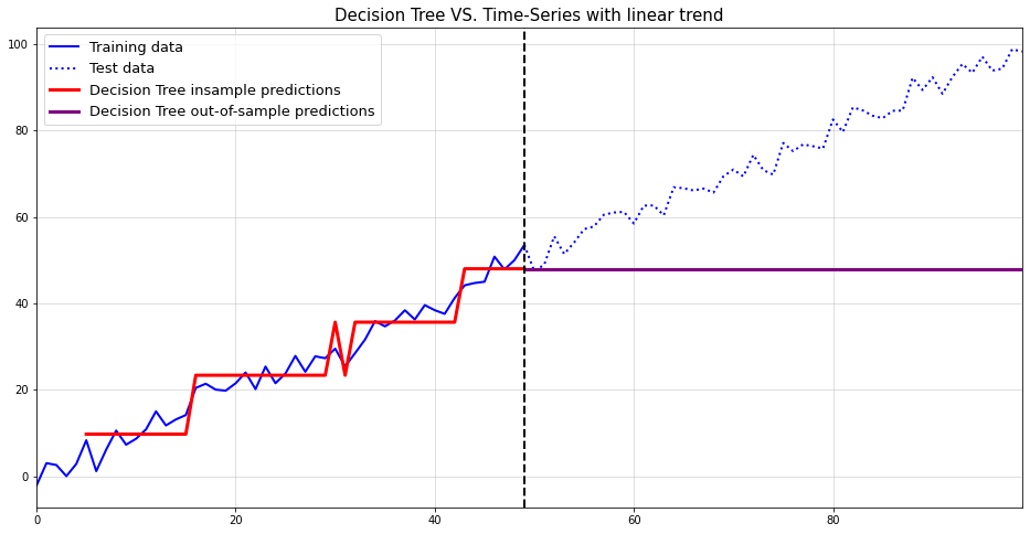
3) Autoregressive Trees cannot handle trends either
import numpy as npimport pandas as pdfrom sklearn.tree import DecisionTreeRegressorimport matplotlib.pyplot as plt#create data with linear trendnp.random.seed(123)t = np.arange(100)y = t +2* np.random.normal(size =100)#linear trendt_train = t[:50].reshape(-1,1)t_test = t[50:].reshape(-1,1)y_train = y[:50]X_train_shift = np.concatenate([pd.Series(y_train).shift(t).values.reshape(-1,1) for t inrange(1,6)],1)[5:,:]y_train_shift = y_train[5:]y_test = y[50:]tree = DecisionTreeRegressor(max_depth =2)tree.fit(X_train_shift, y_train_shift)y_pred_train = tree.predict(X_train_shift).reshape(-1)Xt = np.concatenate([X_train_shift[-1,1:].reshape(1,-1),np.array(y_train_shift[-1]).reshape(1,1)],1)predictions_test = []for t inrange(len(y_test)): pred = tree.predict(Xt) predictions_test.append(pred[0]) Xt = np.concatenate([Xt[-1,1:].reshape(1,-1),np.array(pred).reshape(1,1)],1)y_pred_test = np.array(predictions_test)plt.figure(figsize = (16,8))plt.plot(t_train.reshape(-1), y_train, label ="Training data", color="blue", lw=2)plt.plot(np.concatenate([np.array(t_train[-1]),t_test.reshape(-1)]), np.concatenate([[y_train[-1]],y_test]), label ="Test data", color="blue", ls ="dotted", lw=2)plt.plot(t_train.reshape(-1)[5:], y_pred_train, label ="Decision Tree insample predictions", color="red", lw =3)plt.plot(np.concatenate([np.array(t_train[-1]),t_test.reshape(-1)]), np.concatenate([[y_pred_train[-1]],y_pred_test]), label ="Decision Tree out-of-sample predictions", color="purple", lw=3)plt.grid(alpha =0.5)plt.axvline(t_train[-1], color="black", lw=2, ls="dashed")plt.legend(fontsize=13)plt.title("Decision Tree VS. Time-Series with linear trend", fontsize=15)plt.margins(x=0)
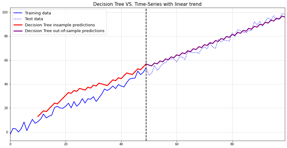
4) Autoregressive Trees can forecast trends if we remove it first
Here, we remove the trend via first-differences
import numpy as npfrom sklearn.tree import DecisionTreeRegressorimport matplotlib.pyplot as plt#create data with linear trendnp.random.seed(123)t = np.arange(100)y = t +2* np.random.normal(size =100)#linear trendt_train = t[:50].reshape(-1,1)t_test = t[50:].reshape(-1,1)n_lags =10y_train = y[:50]X_train_shift = pd.concat([pd.DataFrame(y_train).shift(t) for t inrange(1,n_lags)],1).diff().values[n_lags:,:]y_train_shift = np.diff(y_train)[n_lags-1:]y_test = y[50:]tree = DecisionTreeRegressor(max_depth =1)tree.fit(X_train_shift, y_train_shift)y_pred_train = tree.predict(X_train_shift).reshape(-1)Xt = np.concatenate([X_train_shift[-1,1:].reshape(1,-1),np.array(y_train_shift[-1]).reshape(1,1)],1)predictions_test = []for t inrange(len(y_test)): pred = tree.predict(Xt) predictions_test.append(pred[0]) Xt = np.concatenate([np.array(pred).reshape(1,1),Xt[-1,1:].reshape(1,-1)],1)y_pred_test = np.array(predictions_test)y_pred_train = y_train[n_lags-2]+np.cumsum(y_pred_train)y_pred_test = y_train[-1]+np.cumsum(y_pred_test)plt.figure(figsize = (16,8))plt.plot(t_train.reshape(-1), y_train, label ="Training data", color="blue", lw=2)plt.plot(np.concatenate([np.array(t_train[-1]),t_test.reshape(-1)]), np.concatenate([[y_train[-1]],y_test]), label ="Test data", color="blue", ls ="dotted", lw=2)plt.plot(t_train.reshape(-1)[n_lags:], y_pred_train, label ="Decision Tree insample predictions", color="red", lw =3)plt.plot(np.concatenate([np.array(t_train[-1]),t_test.reshape(-1)]), np.concatenate([[y_pred_train[-1]],y_pred_test]), label ="Decision Tree out-of-sample predictions", color="purple", lw=3)plt.grid(alpha =0.5)plt.axvline(t_train[-1], color="black", lw=2, ls="dashed")plt.legend(fontsize=13)plt.title("Decision Tree VS. Time-Series with linear trend", fontsize=15)plt.margins(x=0)
/var/folders/2d/hl2cr85d2pb2kfbmsng3267c0000gn/T/ipykernel_84684/2778805950.py:16: FutureWarning: In a future version of pandas all arguments of concat except for the argument 'objs' will be keyword-only
  X_train_shift = pd.concat([pd.DataFrame(y_train).shift(t) for t in range(1,n_lags)],1).diff().values[n_lags:,:]
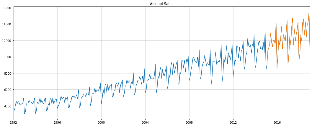
remove yearly seasonlity via 12th-order differencing
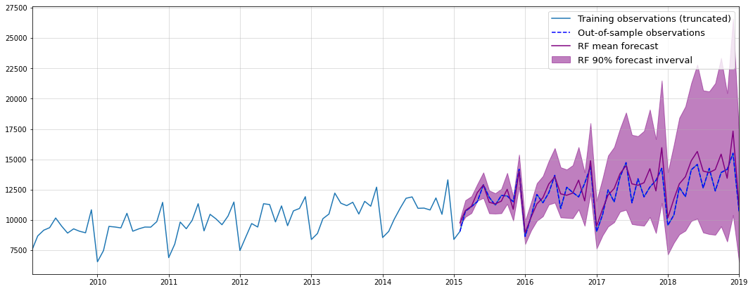
Fit Random Forest model and perform forecast
from sklearn.ensemble import RandomForestRegressorfrom copy import deepcopyclass RandomForestARModel():""" Autoregressive forecasting with Random Forests """def__init__(self, n_lags=1, max_depth =3, n_estimators=1000, random_state =123, log_transform =False, first_differences =False, seasonal_differences =None):""" Args: n_lags: Number of lagged features to consider in autoregressive model max_depth: Max depth for the forest's regression trees random_state: Random state to pass to random forest log_transform: Whether the input should be log-transformed first_differences: Whether the input should be singly differenced seasonal_differences: Seasonality to consider, if 'None' then no seasonality is presumed """self.n_lags = n_lagsself.model = RandomForestRegressor(max_depth = max_depth, n_estimators = n_estimators, random_state = random_state)self.log_transform = log_transformself.first_differences = first_differencesself.seasonal_differences = seasonal_differencesdef fit(self, y):""" Args: y: training data (numpy array or pandas series/dataframe) """#enable pandas functions via dataframes y_df = pd.DataFrame(y)self.y_df = deepcopy(y_df)#apply transformations and store results for retransformationsifself.log_transform: y_df = np.log(y_df)self.y_logged = deepcopy(y_df)ifself.first_differences: y_df = y_df.diff().dropna()self.y_diffed = deepcopy(y_df)ifself.seasonal_differences isnotNone: y_df = y_df.diff(self.seasonal_differences).dropna()self.y_diffed_seasonal = deepcopy(y_df)#get lagged features Xtrain = pd.concat([y_df.shift(t) for t inrange(1,self.n_lags+1)],axis=1).dropna()self.Xtrain = Xtrain ytrain = y_df.loc[Xtrain.index,:]self.ytrain = ytrainself.model.fit(Xtrain.values,ytrain.values.reshape(-1))def sample_forecast(self, n_periods =1, n_samples =10000, random_seed =123):""" Draw forecasting samples by randomly drawing from all trees in the forest per forecast period Args: n_periods: Ammount of periods to forecast n_samples: Number of samples to draw random_seed: Random seed for numpy """ samples =self._perform_forecast(n_periods, n_samples, random_seed) output =self._retransform_forecast(samples, n_periods)return outputdef _perform_forecast(self, n_periods, n_samples, random_seed):""" Forecast transformed observations Args: n_periods: Ammount of periods to forecast n_samples: Number of samples to draw random_seed: Random seed for numpy """ samples = [] np.random.seed(random_seed)for i inrange(n_samples):#store lagged features for each period Xf = np.concatenate([self.Xtrain.iloc[-1,1:].values.reshape(1,-1),self.ytrain.iloc[-1].values.reshape(1,1)],1) forecasts = []for t inrange(n_periods): tree =self.model.estimators_[np.random.randint(len(self.model.estimators_))] pred = tree.predict(Xf)[0] forecasts.append(pred)#update lagged features for next period Xf = np.concatenate([Xf[:,1:],np.array([[pred]])],1) samples.append(forecasts)return samplesdef _retransform_forecast(self, samples, n_periods):""" Retransform forecast (re-difference and exponentiate) Args: samples: Forecast samples for retransformation n_periods: Ammount of periods to forecast """ full_sample_tree = []for samp in samples: draw = np.array(samp)#retransform seasonal differencingifself.seasonal_differences isnotNone: result =list(self.y_diffed.iloc[-self.seasonal_differences:].values)for t inrange(n_periods): result.append(result[t]+draw[t]) result = result[self.seasonal_differences:]else: result = []for t inrange(n_periods): result.append(draw[t])#retransform first differences y_for_add =self.y_logged.values[-1] ifself.log_transform elseself.y_df.values[-1]ifself.first_differences: result = y_for_add + np.cumsum(result)#retransform log transformationifself.log_transform: result = np.exp(result) full_sample_tree.append(result.reshape(-1,1))return np.concatenate(full_sample_tree,1)
Benchmark fitting a kernel density model to the differenced time-series
=> assumes that all autocorrelation has been removed via differencing
=> see also here
from scipy.stats import gaussian_kdekde = gaussian_kde(df_train_trans.values[:,0])target_range = np.linspace(np.min(df_train_trans.values[:,0])-0.5,np.max(df_train_trans.values[:,0])+0.5,num=100)full_sample_toy = [] np.random.seed(123)for i inrange(10000): draw = kde.resample(len(df_test)).reshape(-1) result =list(df_train_diffed.iloc[-12:].values)for t inrange(len(df_test)): result.append(result[t]+draw[t]) full_sample_toy.append(np.exp(np.array((np.log(df_train.values[-1])+np.cumsum(result[12:]))).reshape(-1,1)))predictions_toy = np.concatenate(full_sample_toy,1)means_toy = np.mean(predictions_toy,1)lowers_toy = np.quantile(predictions_toy,0.05,1)uppers_toy = np.quantile(predictions_toy,0.95,1)plt.figure(figsize = (18,7))plt.grid(alpha=0.5)plt.plot(df.iloc[-120:], label ="Training observations (truncated)")plt.plot(df_test, color ="blue", label ="Out-of-sample observations", ls="dashed")plt.plot(df_test.index,means_toy,color="red", label ="Benchmark mean forecast")plt.fill_between(df_test.index, lowers_toy, uppers_toy, color="red", alpha=0.5, label ="Benchmark 90% forecast inverval")plt.legend(fontsize=13)plt.margins(x=0)
---------------------------------------------------------------------------NameError Traceback (most recent call last)
Input In [8], in <cell line: 3>() 1fromscipy.statsimport gaussian_kde
----> 3 kde = gaussian_kde(df_train_trans.values[:,0])
5 target_range = np.linspace(np.min(df_train_trans.values[:,0])-0.5,np.max(df_train_trans.values[:,0])+0.5,num=100)
9 full_sample_toy = []
NameError: name 'df_train_trans' is not defined
plt.figure(figsize = (18,7))plt.grid(alpha=0.5)plt.plot(df.iloc[-120:], label ="Training observations (truncated)")plt.plot(df_test, color ="blue", label ="Out-of-sample observations", ls="dashed")plt.plot(df_test.index,means_tree,color="purple", label ="RF mean forecast",lw =3)plt.plot(df_test.index,means_toy,color="red", label ="Benchmark mean forecast", lw =3)plt.legend(fontsize=13)plt.margins(x=0)